Mapping Forest Change and Carbon Loss in Oregon, 2019 to 2025
Kathryn Wheeler, Ph.D. · Code on GitHub
The goal of this analysis is to investigate land use / land cover (LULC) change in the forested ecoregions of Oregon and to estimate how much aboveground carbon was present in forests before deforestation that occurred between 2019 and 2025.
1. Importance
Oregon's forests are changing quickly and for several reasons at once. Industrial timber harvest cycles through the Coast Range and western Cascades on a few decades' rotation. Stand replacing fire has become larger and more frequent, most dramatically during the Labor Day 2020 event, when several fires ignited within 48 hours and burned hundreds of thousands of acres. Urban and exurban development converts forest along the Willamette Valley margin. Drought and insect mortality thin stands east of the crest without removing them outright.
These changes are not interchangeable ecologically. A clearcut regenerates on a planned schedule. A stand replacing burn resets succession and can shift species composition for a century. Conversion to development removes the forest permanently. Each carries different consequences for habitat connectivity, for water yield and stream temperature, and for the carbon the landscape holds.
This project is most interested in carbon. Standing forest holds carbon in living biomass; when forest is lost, most of that carbon is eventually released. Knowing how much area changed, and how much carbon that area was holding, is what converts a land cover map into an emissions estimate.
Why build a regional model when global products exist
Global land cover and forest change products are widely used and well validated at global scale. But a model fit to the whole planet must compromise: the spectral signature that separates forest from shrubland in the tropics is not the one that separates a young Douglas fir plantation from regenerating shrub in the Coast Range. Accuracy that is acceptable globally can be poor in any particular place. Training on regional reference data addresses this directly. The tradeoff is that regional labels are scarce and expensive, which is the constraint that shapes much of what follows.
2. The data
GLanCE: the reference labels
GLanCE (Global Land Cover Estimation, Boston University) is a globally distributed set of human interpreted land cover reference points, each a location with a land cover class and a time span over which that class held, built by analysts reading Landsat time series and high resolution imagery. This analysis uses the 48,014 North America records, exploded into one row per location per year over 2017 to 2025. Labels stop in 2021, which is why the 2025 map is treated as extrapolation and flagged as such throughout. Only about 2,247 points fall in the Pacific Northwest, far too few to train on alone, so models are trained across all of North America and then tested specifically on Washington and Oregon points to confirm they transfer.
AlphaEarth: the predictors
Rather than feed raw satellite reflectance to a classifier, this analysis uses AlphaEarth Satellite Embeddings, a Google DeepMind product available in Earth Engine. For every 10 m pixel and every year from 2017, AlphaEarth provides a 64 number summary of everything the satellites saw at that location that year, learned by a foundation model trained on optical, radar, and lidar observations. Two pixels with similar vegetation, structure, and seasonality end up with similar numbers, which means the hard sensing work (cloud gaps, sensor differences, seasonal timing, multi-sensor fusion) is already done, and that comparing a pixel's 2019 and 2025 embeddings is itself a change signal, which is what the change model in Section 9 exploits.
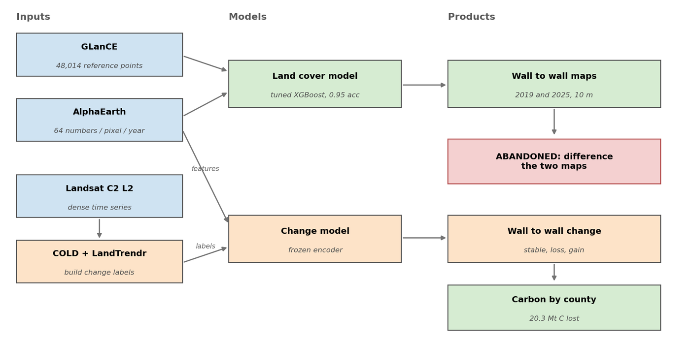
The two branches are the story. The upper path (classify each year, then difference) was built, measured, and set aside. The lower path predicts change directly and is what determines the carbon number.
3. Classifying land cover
The first task is a per-pixel land cover classifier: given a pixel's 64 AlphaEarth numbers for a year, predict its GLanCE Level 1 class (water, developed, barren, trees, shrubs, herbaceous). Nine model variants were compared under identical conditions, from tree ensembles through neural networks, including a CNN that sees a pixel's neighborhood rather than the pixel alone. Points from the same GLanCE segment always land in the same cross-validation fold, so a model cannot be scored on a location it was fit on, and a separate evaluation holds out Washington and Oregon points entirely.
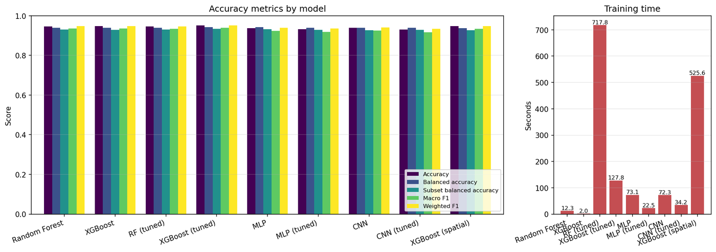
A tuned gradient boosted tree (XGBoost) won, at 0.950 accuracy overall. On the held-out Washington and Oregon points it reaches 0.938, confirming that a model trained across all of North America transfers to the target region. The neural networks did not beat it, which is worth stating plainly because it is the opposite of the usual expectation: AlphaEarth already did the representation learning, so once a pixel is described by 64 well separated numbers, the remaining task is ordinary tabular classification, and gradient boosted trees are extremely good at that.
4. Pilot: the Labor Day 2020 fires
Before committing to a state sized run, the whole chain was tested on one event with independently known answers: the Holiday Farm Fire on the McKenzie River, which ignited September 8, 2020, and burned about 70,600 ha. The point of a pilot on a known disturbance, rather than an arbitrary patch, is that it tests the science and not just the plumbing. Fire severity from MTBS gives a quantitative expectation: within the perimeter, MTBS records roughly 9% unburned, 27% low, 30% moderate, and 33% high severity. Low severity underburn leaves the canopy standing, so those pixels are still forest; only stand replacing fire should flip the land cover class. A change map that flags the entire perimeter is over-detecting; one that flags about a third is behaving correctly.
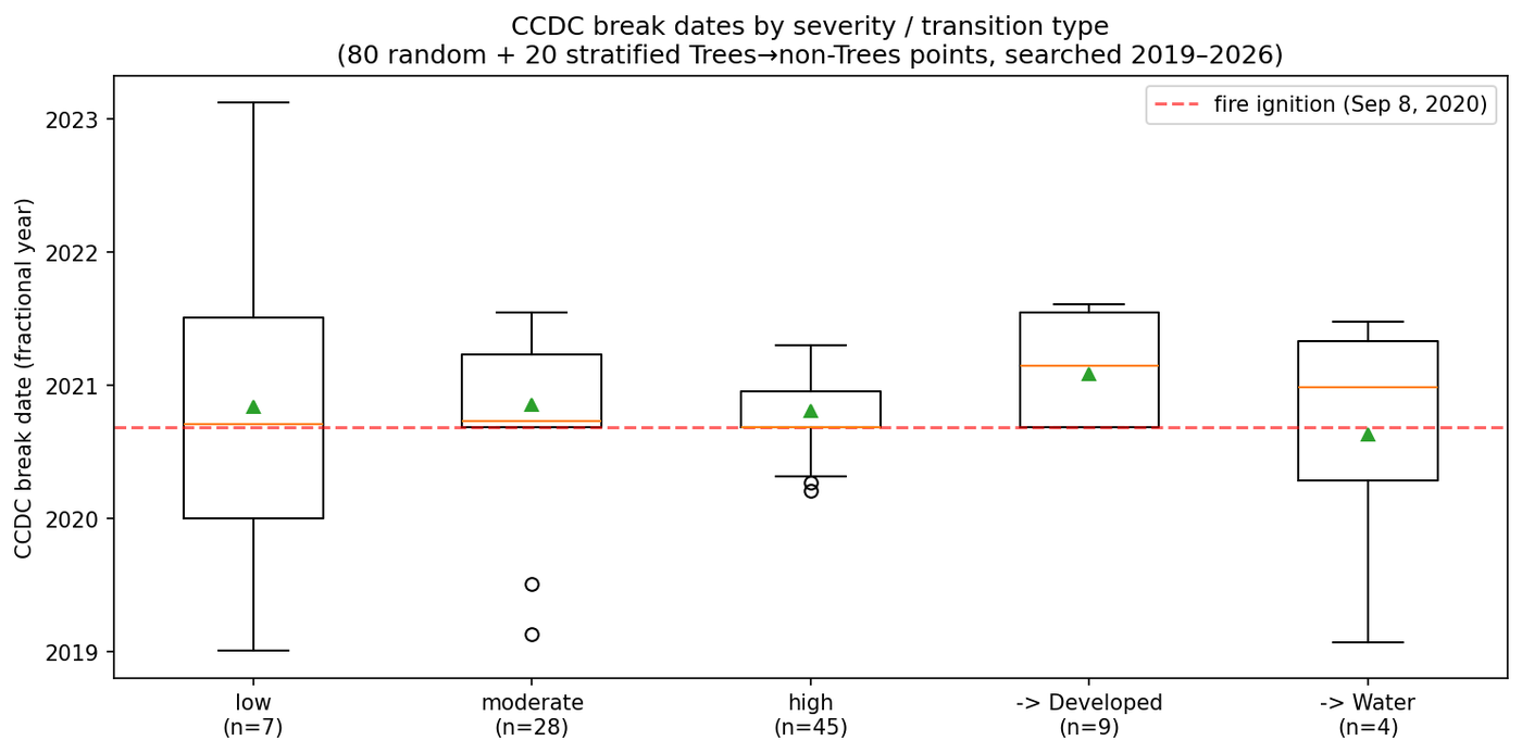
The pilot also confirmed that break dates land in September 2020, that the fire splits sensibly across county lines with no double counting at the border, and that containerized inference produces identical predictions locally and on the cloud VM. One reconciliation problem surfaced here and is worth flagging: MTBS's reported acreage did not initially match the area computed from its own polygon, a gap of roughly 39%. Discrepancies of that kind silently corrupt area-based carbon numbers, and finding it in a pilot rather than in a state wide run is precisely why the pilot existed.
5. Choosing a change detection algorithm: COLD over CCDC
The pilot also settled which time series algorithm would date change for the rest of the project. Because the Holiday Farm ignition date is known exactly, the fire is a natural benchmark: any algorithm claiming to date disturbance should land on that day. CCDC (Continuous Change Detection and Classification) is the established method and runs natively inside Earth Engine. COLD (Zhu et al. 2020) is its faster successor but runs locally through the pyxccd library. The test used 50 points: 30 drawn at random from mapped Trees to non-Trees change, plus 20 deliberate false-positive bait points (Trees to Water, Trees to Developed) that a good algorithm should decline to date.
| Method | Breaks found | Dated within 25 days | Median error |
|---|---|---|---|
| CCDC, default | 36 / 50 | 15 | 176 days |
| CCDC, tuned | 41 / 50 | 22 | 8 days |
| COLD, default | 42 / 50 | 23 | 8 days |
| COLD, tuned | 45 / 50 | 30 | 1 day |
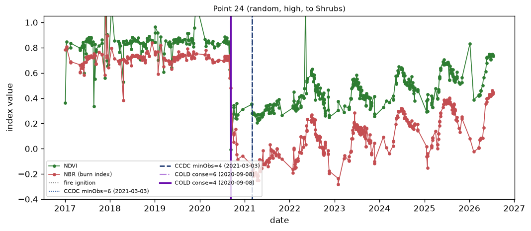
An unambiguous high severity fire pixel. Both COLD settings date it to the exact ignition day; both CCDC settings lag by roughly six months.
COLD dated the fire markedly closer at every matched setting, with no increase in spurious pre-fire breaks. Tuned COLD put 30 of 50 points within 25 days of ignition against 22 for tuned CCDC, with a median error of a single day. CCDC costs about five to six seconds per point, almost all of it a round trip to Earth Engine; COLD pays a similar one-time cost to extract Landsat observations, but then runs in about seven milliseconds per point, roughly a thousand times faster once the data is local. That speed is what made it practical to run COLD across all 13,000 reference points and sweep its settings.
This is one fire and one disturbance type, which tests abrupt disturbance dating specifically, so the labelling pipeline in Section 8 adds two independent trend based methods rather than relying on COLD alone. Full detail, including the per-point break table, is in COLD_vs_CCDC_Comparison.md in the project repository.
6. Wall to wall land cover, 2019 and 2025
The classifier was run across every forested pixel in Oregon for both years: twelve hand-picked ecoregions from RESOLVE Ecoregions 2017, intersected with the Oregon boundary, covering the Coast Range, Cascades, Klamath Siskiyou, Blue Mountains, and the Willamette Valley oak savanna, while excluding shrub steppe, desert, and glaciers. At 171,329 km² at 10 m resolution, that is about 1.71 billion pixels, and the 64-band embeddings come to roughly 0.44 TB per year, which does not fit on a laptop. The embeddings were exported to cloud storage, the trained model was packaged into a container, and inference ran on a temporary virtual machine in the same region.
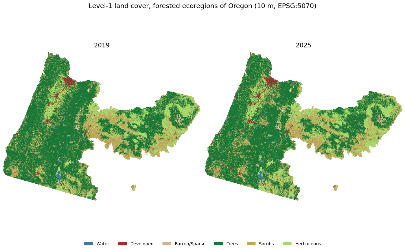
One caveat carried forward throughout: GLanCE labels end in 2021, so the 2025 map is out of sample for the classifier and every downstream use of it inherits that limitation.
7. Where the conventional approach broke down
With two maps in hand, a natural next step is to difference them: any pixel whose class differs between 2019 and 2025 is change. This is standard practice, and here it failed. Each map is about 95% accurate, but the two maps make mistakes independently, so a pixel is flagged as changed whenever either map is wrong about it. Roughly 10% of pixels can disagree from classifier error alone, while genuine land cover change over six years affects only a few percent of the landscape. The noise is larger than the signal.
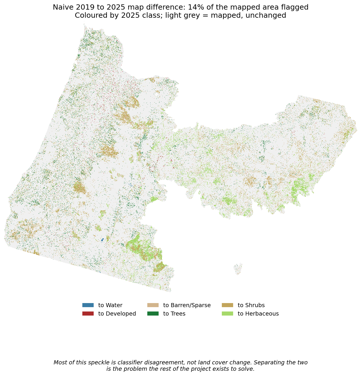
The naive difference flagged 2.38 million hectares as changed, of which only about 8% carried high confidence from both years. Feeding this into a carbon calculation would have produced a large, confident, and badly wrong number. This is a well known trap in post-classification comparison, and the project's response was to stop treating the difference as an answer. It became at most a candidate mask, and was eventually replaced entirely by the change model in Section 9.
8. Building trustworthy change labels
To train a model to recognize change directly, labels are needed: locations where it is known whether change happened, in which direction, and when. GLanCE cannot supply these at the density required in Oregon, so they were built. A probability sample of 13,000 points was drawn across the study area, stratified so that both candidate change and apparently stable areas are represented. Each point's full Landsat time series was then analyzed with three independent methods: COLD (abrupt events such as fire and harvest), a model-free NDVI trend test (Theil-Sen slope with Mann-Kendall significance, for gradual change break detectors miss), and LandTrendr (multi-year decline and recovery).
Each point is labelled stable, increase, or decrease, with the direction taken from whichever signal dominates. A confidence score combines agreement across the three methods, margin past each threshold, consistency with the mapped transition, and corroboration from Hansen forest loss year. High confidence labels are accepted automatically; low confidence ones are reviewed by reading the time series panel by panel, initially by an LLM (Claude Sonnet) and spot-checked by hand. Across 299 points reviewed for the accuracy assessment, agreement with the automated label ran near 100% in the high confidence tier but only 51% to 59% in the low tier, exactly the pattern the confidence score was designed to predict.
9. A model that sees change directly
The change model takes a pixel's 2019 and 2025 embeddings together as a single input and predicts stable, increase, or decrease. Because it never forms two independent maps, it cannot compound their errors; it learns what a genuine before and after transition looks like, rather than comparing two annual snapshots that merely differ. Five architectures were compared, and the winner freezes the land cover classifier already trained on GLanCE so it cannot change, then trains only a small new head that reads its internal representation of both years and decides whether change occurred. Freezing matters: it means the change labels, the noisier of the two label sources, cannot corrupt what the model knows about land cover.
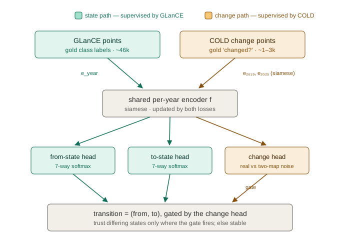
The frozen encoder was selected on balanced accuracy (0.956) and subset balanced accuracy (0.961) rather than raw accuracy, since the landscape is overwhelmingly stable and a model that predicted "no change" everywhere would still score well on plain accuracy. These metrics average performance across classes and across the change classes only, so they measure the thing the map exists to find. The frozen encoder also trains in about a quarter of the time of the tree-based alternative.
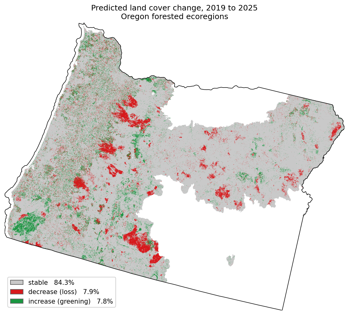
17,163,110 ha mapped: 84.3% stable, 7.9% decrease (loss), 7.8% increase (greening). Loss concentrates where it should, in the 2020 fire scars in the western Cascades and harvest units in the Coast Range; gain is mostly regrowth on older disturbance.
10. How accurate is it, and is it actually better
Accuracy was assessed against 396 reference points the change model never saw during training, using a design based estimator that weights each point by how much of the landscape its stratum represents (Olofsson et al. 2014). Of 397 verified points available, 279 had trained the model and were excluded; 299 fresh points were reviewed by hand to rebuild the sample, then used to score the naive map difference too, so the two are separated by nothing except which map is being judged.
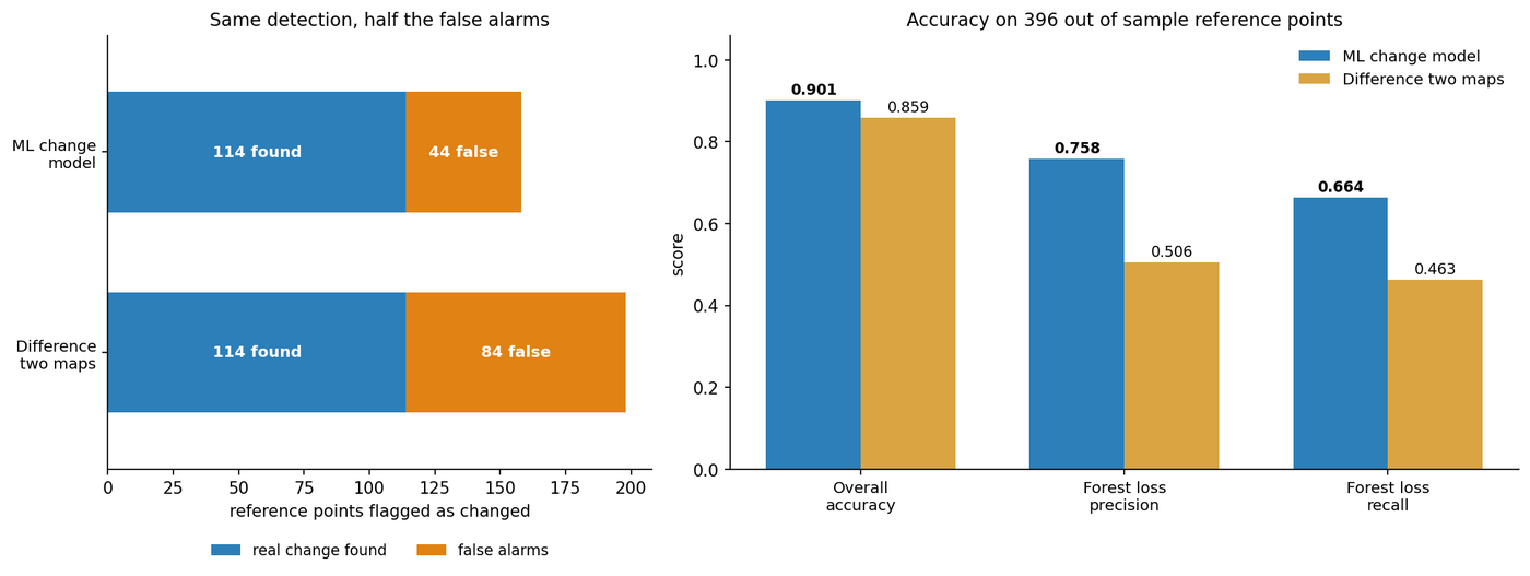
Of 144 reference points that genuinely changed, both approaches found 114 and missed 30: detection is identical. But getting there, the naive difference raised 84 false alarms against the model's 44. The improvement is almost entirely a halving of false positives, not better sensitivity. Overall accuracy improves by only 0.04, because both approaches are over 90% correct on the stable class that covers 84% of the landscape, but precision on forest loss, the quantity carbon depends on, improves by 0.25: half of what the naive map calls deforestation is not deforestation, versus about a quarter for the ML map.
A map's pixel count is a biased estimate of true area, because commission and omission errors do not cancel. The design based estimator corrects this: forest loss is undercounted by 12.4%, so the corrected area is higher than the raw pixel count, while forest gain is overcounted by 27%.
Everything above is an internal check. The reference labels and the map both read the same Landsat and AlphaEarth record, so a high score shows the pipeline is coherent, not that it is right about Oregon. Hansen Global Forest Change is an outside answer, built by other people from a different algorithm on a 30 m grid, and over the identical study area it puts 2019 to 2025 forest loss between 861,988 and 1,107,799 ha. That range is a bracket rather than a single number because two choices are genuinely ambiguous: whether loss during 2019 counts, since it is already partly visible in the 2019 embedding the model read, and whether Hansen is restricted to pixels holding at least 30% tree cover in 2000, since it otherwise flags loss on sparse woodland this map never called forest.
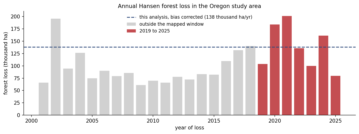
This analysis puts the figure at 827,886 ha, or 1.37% per year of the 10.09 million ha it classified as forest in 2019. Three of the four Hansen variants fall inside its 95% confidence interval, and the closest analogue, the strict 2020 to 2025 window restricted to at least 30% cover, sits 4% above at 861,988 ha. Two products sharing no algorithm and no input pipeline landing this close is the strongest evidence here that the area estimate is right rather than merely self consistent. This map does read slightly low against all four variants, which is what a stricter definition of forest would predict. The 2020 and 2021 spikes are the Labor Day fires, split across two loss years because Hansen confirms late season loss in the following year's imagery, which is why a six year mean is the honest unit here rather than any single year.
11. From area to carbon
The carbon present before deforestation is estimated as activity data times emission factor, the standard accounting form: hectares of forest lost in a county, times aboveground biomass density for that county, times 0.47 to convert biomass to carbon. Forest loss is defined conservatively, requiring two independent lines of evidence to agree (the land cover maps show trees becoming non-trees, and the change model independently calls that pixel a decrease); the naive candidate covered 954,493 ha, and requiring confirmation retains 725,168 ha, or 76%. Biomass density comes from USDA Forest Inventory and Analysis county level estimates, which carry published sampling errors, which is what makes a genuine uncertainty interval possible.
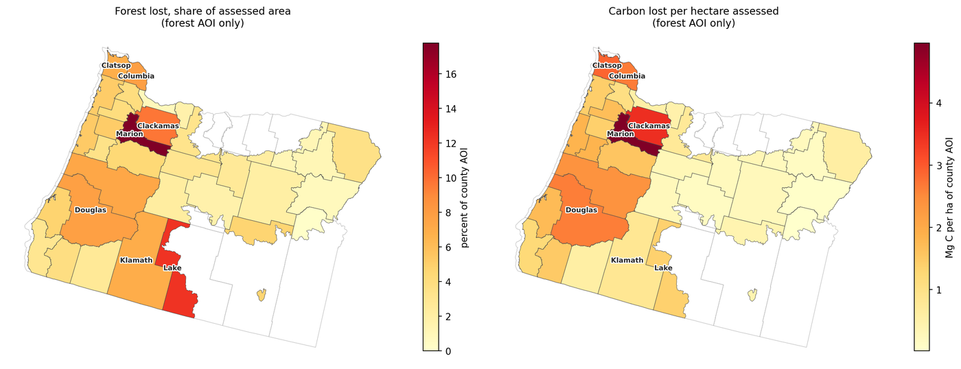
The result is 20.3 million Mg C, with a 95% confidence interval of 14.2 to 26.4 million. The interval combines uncertainty in how much area was really lost (15.1%, from the accuracy assessment) and uncertainty in biomass density (2.7%, from FIA); area dominates, so reporting only the FIA error, as is common, would have implied an interval roughly six times too narrow.
Area and carbon are not the same map: biomass density across the study area ranges from about 24 to 89 Mg per hectare, a threefold spread. Marion County is the intensity outlier, dark in both panels, at 17.8% of its assessed forest lost and 4.96 Mg C per hectare, roughly double any other county. Lake County shows the density effect clearly, strongly colored on area lost (12.3%) yet pale on carbon, because its forest holds only about 24 Mg per hectare. Douglas County is mid-toned in both panels yet releases the most carbon of any county (3.45 million Mg C) through sheer size rather than intensity. Ranking counties by area alone would have pointed at the wrong places.
12. What this analysis supports, and what it does not
Supported
- A regionally trained classifier reaches 0.95 accuracy on Oregon forest land cover and transfers from continental training data to the target region without local retraining.
- Predicting change directly beats differencing two classified maps, with the gain specifically in precision on forest loss (+0.25), measured on points neither model had seen.
- Forest loss over 2019 to 2025 is 827,886 ha bias corrected, carrying 20.3 million Mg C, with an interval that prices both area and emission factor uncertainty.
- Where matters as much as how much: threefold variation in biomass density means area and carbon rankings genuinely differ across counties.
- The rate holds up against an independent product. Hansen Global Forest Change brackets the same window at 861,988 to 1,107,799 ha over the identical footprint, and three of its four variants fall inside this analysis's confidence interval.
Not supported, and why
- This is canopy loss, not deforestation in the sense a carbon methodology means. In Oregon the signal is dominated by rotational harvest and by wildfire, and harvested or burned land remains forest land use because it regrows. Establishing deforestation would need a persistence test on the land use, which neither this analysis nor Hansen performs. What this produces is the activity data layer such a test consumes, with its uncertainty already quantified.
- The 2025 map is extrapolation. GLanCE labels end in 2021, so nothing here validates the classifier's 2025 output against contemporaneous truth.
- Only change direction is independently verified. What a pixel changed from and to still comes from the classifier's own predictions, so restricting to tree loss inherits that model's error; the correction is a uniform ratio rather than a class-specific estimate.
- Forest gain is the weak class, at 0.53 precision: roughly half of mapped greening is not real.
- Carbon is aboveground only (soil, roots, and dead wood are excluded) and is not a net figure, since regrowth elsewhere is mapped but not subtracted. These are estimates of carbon present before deforestation, likely greater than the amount actually lost, and county mean emission factors mix young and mature forest, so carbon per hectare here sits below what a mature stand would give.
Judgment calls that shaped the result
- Abandoning map differencing. Keeping it would have produced a confident, large, and wrong answer.
- Excluding 279 contaminated reference points and reviewing 299 fresh ones. The contaminated version would have reported optimistic accuracy and a wrong correction factor.
- Piloting on a fire with independently known severity, which turned validation into a falsifiable prediction rather than a visual impression.
Where to find things
| Notebook | What it contains |
|---|---|
| Classification_Model_Selection.ipynb | GLanCE loading, embedding sampling, and the nine-way land cover model comparison |
| Pilot_LaborDayFires.ipynb | Holiday Farm Fire end-to-end test against MTBS severity |
| Wall_to_Wall_Maps.ipynb | AOI construction, cloud export and inference, the 13,000-point reference sample, COLD labelling |
| Change_Model_Selection.ipynb | The five-way change model comparison, including the map differencing baseline |
| Wall_to_Wall_Change_Maps.ipynb | Change map production, accuracy assessment, the Hansen benchmark, and carbon accounting |
Full code and supporting write-ups, including COLD_vs_CCDC_Comparison.md and setup instructions, are on GitHub.